Proton Calorimetry/Equipment/Caen Detector Emulator: Difference between revisions
SimonJolly (talk | contribs) No edit summary |
SimonJolly (talk | contribs) No edit summary |
||
| (10 intermediate revisions by the same user not shown) | |||
| Line 13: | Line 13: | ||
To generate a spectrum for use with the detector emulator, the sample waveforms need to intergrated and put into a histogram. See the figures below shwo an example waveform, a sample of waveforms from a single data file and a generated histogram respectively. If the spectrum is generated as described, from oscilloscope data, the bin width needs to recorded so that the spectrum can be scaled accordingly via the emulator software interface. | To generate a spectrum for use with the detector emulator, the sample waveforms need to intergrated and put into a histogram. See the figures below shwo an example waveform, a sample of waveforms from a single data file and a generated histogram respectively. If the spectrum is generated as described, from oscilloscope data, the bin width needs to recorded so that the spectrum can be scaled accordingly via the emulator software interface. | ||
<div class="image600px">http://www.hep.ucl.ac.uk/pbt/wikiData/images/CaenDetectorEmulator/single_wf_20kHz.jpg</div> | <div class="image600px">[http://www.hep.ucl.ac.uk/pbt/wikiData/images/CaenDetectorEmulator/single_wf_20kHz.jpg http://www.hep.ucl.ac.uk/pbt/wikiData/images/CaenDetectorEmulator/single_wf_20kHz.jpg]</div> | ||
<div class="image600px">http://www.hep.ucl.ac.uk/pbt/wikiData/images/CaenDetectorEmulator/C1Trace00000.png</div> | <div class="image600px">[http://www.hep.ucl.ac.uk/pbt/wikiData/images/CaenDetectorEmulator/C1Trace00000.png http://www.hep.ucl.ac.uk/pbt/wikiData/images/CaenDetectorEmulator/C1Trace00000.png]</div> | ||
<div class="image600px">http://www.hep.ucl.ac.uk/pbt/wikiData/images/CaenDetectorEmulator/1.98mmCol_RateTest_20kHz_fullSpectrum.jpg</div> | <div class="image600px">[http://www.hep.ucl.ac.uk/pbt/wikiData/images/CaenDetectorEmulator/1.98mmCol_RateTest_20kHz_fullSpectrum.jpg http://www.hep.ucl.ac.uk/pbt/wikiData/images/CaenDetectorEmulator/1.98mmCol_RateTest_20kHz_fullSpectrum.jpg]</div> | ||
=== Spectrum Modifications === | === Spectrum Modifications === | ||
Ideally the method used to create the spectrum should be able to detect bad waveforms, such as those where pile-up has occurred, and discard them so that an | Ideally the method used to create the spectrum should be able to detect bad waveforms, such as those where pile-up has occurred, and discard them so that an "ideal" spectrum is generated. This is so that the these features can be replicated more realistically using the emulator rather than just leaving the artefacts in the spectrum. For example, if the secondary peak from pile-up is in the spectrum, the emulator will take this as part of the “main” spectrum and simply generate pulses with double the area to recreate this secondary peak. To remove some of the bad pulses, a rather primitive method was used to remove that formed part of the spectrum beyond the Gaussian peak and Landau tail. This in effect removed the majority of the additional peaks from pile-up or that were abnormally large. | ||
In order for the position of the spectra to be correct, in terms of ADC channel, the file containing the spectral shape needs to start from 0, i.e. if the first populated bin is at 5000 pVs then all prior unpopulated bins from 0 pVs to 5000 pVs need to be included in the spectrum file. Furthermore, it was observed that the x-axis of the spectrum should be scaled using the software interface when importing so that the spectrum is wide enough so that the finer details of the spectrum are reproduced. The simplest two ways to ensure the correct scale along this axis are to either scale by the histogram bin width or to chose a bin width of 1 pVs when producing the spectral histogram. It was found to be best practice not to scale the spectrum along the y-axis (adjusting the peak), as this will exacerbate the features of the spectrum rendering the emulation inaccurate. An example of the adjusted and modified spectrum can be seen in the figure below. | In order for the position of the spectra to be correct, in terms of ADC channel, the file containing the spectral shape needs to start from 0, i.e. if the first populated bin is at 5000 pVs then all prior unpopulated bins from 0 pVs to 5000 pVs need to be included in the spectrum file. Furthermore, it was observed that the x-axis of the spectrum should be scaled using the software interface when importing so that the spectrum is wide enough so that the finer details of the spectrum are reproduced. The simplest two ways to ensure the correct scale along this axis are to either scale by the histogram bin width or to chose a bin width of 1 pVs when producing the spectral histogram. It was found to be best practice not to scale the spectrum along the y-axis (adjusting the peak), as this will exacerbate the features of the spectrum rendering the emulation inaccurate. An example of the adjusted and modified spectrum can be seen in the figure below. | ||
<div class="image600px">http://www.hep.ucl.ac.uk/pbt/wikiData/images/CaenDetectorEmulator/1.98mmCol_RateTest_20kHz_trim.jpg</div> | <div class="image600px">[http://www.hep.ucl.ac.uk/pbt/wikiData/images/CaenDetectorEmulator/1.98mmCol_RateTest_20kHz_trim.jpg http://www.hep.ucl.ac.uk/pbt/wikiData/images/CaenDetectorEmulator/1.98mmCol_RateTest_20kHz_trim.jpg]</div> | ||
== Signal Shape Emulation == | == Signal Shape Emulation == | ||
| Line 29: | Line 29: | ||
The detector emulator allows the user to customise the shape of the output signal pulse. The user can choose to either use the default exponential decay pulse, to define their own custom shape from a list of predefined modifiable inbuilt shapes or shape from an imported .csv file. In addition there is also the ability to generate a multi-shape pulse consisting of two defined signal shapes. In the evaluation of the detector emulator all of the inbuilt signal shapes were tested, these are suitable for simple emulations or in driving additional hardware such as an LED. As one of the aims of the evaluation was to emulate experiential data, an “ideal” waveform was produced from experimental for use with the detector emulator. | The detector emulator allows the user to customise the shape of the output signal pulse. The user can choose to either use the default exponential decay pulse, to define their own custom shape from a list of predefined modifiable inbuilt shapes or shape from an imported .csv file. In addition there is also the ability to generate a multi-shape pulse consisting of two defined signal shapes. In the evaluation of the detector emulator all of the inbuilt signal shapes were tested, these are suitable for simple emulations or in driving additional hardware such as an LED. As one of the aims of the evaluation was to emulate experiential data, an “ideal” waveform was produced from experimental for use with the detector emulator. | ||
=== Generating an | === Generating an "Ideal" Waveform === | ||
Although a signal from a PMT can be roughly characterised using a single or exponential equation, finding the parameters from fitting a function to characterise a typical signal from a specific data set would not straight forward due to the energy/area distribution of the unmodified spectra. Therefore, the chosen method to generate an ideal waveform/signal was to take a selection of “good” waveforms and produce an average signal from them. | Although a signal from a PMT can be roughly characterised using a single or exponential equation, finding the parameters from fitting a function to characterise a typical signal from a specific data set would not straight forward due to the energy/area distribution of the unmodified spectra. Therefore, the chosen method to generate an ideal waveform/signal was to take a selection of “good” waveforms and produce an average signal from them. | ||
| Line 39: | Line 39: | ||
This averaging created a waveform that had the same time resolution as the original data recorded by the oscilloscope which was found to be far finer than what the detector emulator ws able to reproduce. Since the shape file does not have a column representing the time values of each data points, it was necessary to create a new shape file that has the data points from the average waveform mapped onto its coarser time resolution. The resolution/time-step for imported signal shapes is not directly stated in the detector emulator user manual. This was simply calculated by dividing the maximum length a signal shape could be by the maximum number of points that the the signal shape can be defined by and found to be 6.348 ns. A comparison between a ”good” average waveform with the resolution of the oscilloscope and a waveform with the data points mapped to the resolution of the detector emulator can be seen in the figure below. | This averaging created a waveform that had the same time resolution as the original data recorded by the oscilloscope which was found to be far finer than what the detector emulator ws able to reproduce. Since the shape file does not have a column representing the time values of each data points, it was necessary to create a new shape file that has the data points from the average waveform mapped onto its coarser time resolution. The resolution/time-step for imported signal shapes is not directly stated in the detector emulator user manual. This was simply calculated by dividing the maximum length a signal shape could be by the maximum number of points that the the signal shape can be defined by and found to be 6.348 ns. A comparison between a ”good” average waveform with the resolution of the oscilloscope and a waveform with the data points mapped to the resolution of the detector emulator can be seen in the figure below. | ||
<div class="image600px">http://www.hep.ucl.ac.uk/pbt/wikiData/images/CaenDetectorEmulator/1.98mmCol_RateTest_20kHz_Sc50_ResCompare.jpg</div> | <div class="image600px">[http://www.hep.ucl.ac.uk/pbt/wikiData/images/CaenDetectorEmulator/1.98mmCol_RateTest_20kHz_Sc50_ResCompare.jpg http://www.hep.ucl.ac.uk/pbt/wikiData/images/CaenDetectorEmulator/1.98mmCol_RateTest_20kHz_Sc50_ResCompare.jpg]</div> | ||
=== Changing Units === | === Changing Units === | ||
| Line 47: | Line 47: | ||
=== Further Modifications === | === Further Modifications === | ||
The imported signal shape was further modified by removing data points (trimming) associated with the dead-time surrounding signal recorded by the oscilloscope (i.e. before trigger and after the pulse). These values which were near to 0 mV (not exactly 0 mV due to dark current) needed to removed so that they were not counted as part of the emulated signal. If left in, this would inhibit the ability to follow the energy spectrum and implement some artificial noise (in particular pile-up). The dark current also had to be subtracted from each of the data points as otherwise, after scaling during emulation, the tail of the signal would form a plateau not tending to 0 mV. The baseline of the average signal was also adjusted so that it was | The imported signal shape was further modified by removing data points (trimming) associated with the dead-time surrounding signal recorded by the oscilloscope (i.e. before trigger and after the pulse). These values which were near to 0 mV (not exactly 0 mV due to dark current) needed to removed so that they were not counted as part of the emulated signal. If left in, this would inhibit the ability to follow the energy spectrum and implement some artificial noise (in particular pile-up). The dark current also had to be subtracted from each of the data points as otherwise, after scaling during emulation, the tail of the signal would form a plateau not tending to 0 mV. The baseline of the average signal was also adjusted so that it was ~0 mV and no longer the opposite polarity of the signal pulse. | ||
=== Final Scaling === | === Final Scaling === | ||
| Line 57: | Line 57: | ||
The time distribution of signals generated by the detector emulator can be defined by one or four separate methods; at a constant rate, with a Poisson distribution, a custom user defined distribution or custom user defined sequence of events. Since the sample sequence mode on the oscilloscope was used to record record experiential data, the exact rate and time distribution of the experimental data could not be determined. Therefore, for the testing/evaluation of the custom distribution and sequence time distribution modes, arbitrary distributions and sequences were used to verify how these modes worked. | The time distribution of signals generated by the detector emulator can be defined by one or four separate methods; at a constant rate, with a Poisson distribution, a custom user defined distribution or custom user defined sequence of events. Since the sample sequence mode on the oscilloscope was used to record record experiential data, the exact rate and time distribution of the experimental data could not be determined. Therefore, for the testing/evaluation of the custom distribution and sequence time distribution modes, arbitrary distributions and sequences were used to verify how these modes worked. | ||
A more in depth evaluation of the constant rate and Poisson time distribution methods was undertaken. These both worked as expected, however it should be noted that the constant rate is defined in terms of kilo counts per second (kcps) where this is equivalent to kHz (i.e. | A more in depth evaluation of the constant rate and Poisson time distribution methods was undertaken. These both worked as expected, however it should be noted that the constant rate is defined in terms of kilo counts per second (kcps) where this is equivalent to kHz (i.e. <span class="nowrap;">1 kips ≡ 1 kHz). | ||
== Emulator Output == | == Emulator Output == | ||
For each iteration of testing the various features of the detector emulator, the signal was output to the Teledyne LeCroy HDO6104 oscilloscope. By using the inbuilt oscilloscope mathematics and graphing functions, it was possible to quickly inspect the output by eye to evaluate if the detector emulator was behaving as expected. The most commonly used inbuilt function/multi-function was to produce an on-the-fly histogram of the signal area. An example of this function in practice can be seen in the figure below, where an | For each iteration of testing the various features of the detector emulator, the signal was output to the Teledyne LeCroy HDO6104 oscilloscope. By using the inbuilt oscilloscope mathematics and graphing functions, it was possible to quickly inspect the output by eye to evaluate if the detector emulator was behaving as expected. The most commonly used inbuilt function/multi-function was to produce an on-the-fly histogram of the signal area. An example of this function in practice can be seen in the figure below, where an ''acceptable'' emulation of the experimental data from the ''1.98mmCol_RateTest_20kHz'' run at the Clatterbridge Cancer Centre, 02/08/2016 with all fo the the above described manipulations applied to the spectrum and signal shape. | ||
<div class="image600px">http://www.hep.ucl.ac.uk/pbt/wikiData/images/CaenDetectorEmulator/AreaHist50kwf_Poisson_1000kHz.png</div> | <div class="image600px">[http://www.hep.ucl.ac.uk/pbt/wikiData/images/CaenDetectorEmulator/AreaHist50kwf_Poisson_1000kHz.png http://www.hep.ucl.ac.uk/pbt/wikiData/images/CaenDetectorEmulator/AreaHist50kwf_Poisson_1000kHz.png]</div> | ||
A comparison between the histogram output from the oscilloscope with the corresponding raw binned experimental data (not adjusted for time-step) can be seen in the two figures below, where both histograms have the same bins. Both histograms have the same shape implying the emulation is accurate however it can be seen that the histogram for the experimental data is shifted to the left, this is expected as the integration does not account for the negative baseline voltage and the integration gates are wider. As mentioned earlier, the negative baseline as been taken into account for the emulation, all be it in a relatively crude manner, when generating the average ``good" waveform shape. | A comparison between the histogram output from the oscilloscope with the corresponding raw binned experimental data (not adjusted for time-step) can be seen in the two figures below, where both histograms have the same bins. Both histograms have the same shape implying the emulation is accurate however it can be seen that the histogram for the experimental data is shifted to the left, this is expected as the integration does not account for the negative baseline voltage and the integration gates are wider. As mentioned earlier, the negative baseline as been taken into account for the emulation, all be it in a relatively crude manner, when generating the average ``good" waveform shape. | ||
<div class="image600px">http://www.hep.ucl.ac.uk/pbt/wikiData/images/CaenDetectorEmulator/500bin_rawData_Comp.jpg</div> | <div class="image600px">[http://www.hep.ucl.ac.uk/pbt/wikiData/images/CaenDetectorEmulator/500bin_rawData_Comp.jpg http://www.hep.ucl.ac.uk/pbt/wikiData/images/CaenDetectorEmulator/500bin_rawData_Comp.jpg]</div> | ||
<div class="image600px">http://www.hep.ucl.ac.uk/pbt/wikiData/images/CaenDetectorEmulator/Hist_sum_emulatorNormal.jpg</div> | <div class="image600px">[http://www.hep.ucl.ac.uk/pbt/wikiData/images/CaenDetectorEmulator/Hist_sum_emulatorNormal.jpg http://www.hep.ucl.ac.uk/pbt/wikiData/images/CaenDetectorEmulator/Hist_sum_emulatorNormal.jpg]</div> | ||
== Noise and Interference Emulation == | == Noise and Interference Emulation == | ||
Artificial noise and interference can applied to an emulation, this is programmable within the detector emulator software interface. These programmable features are: random number noise, white noise, | Artificial noise and interference can applied to an emulation, this is programmable within the detector emulator software interface. These programmable features are: random number noise, white noise, ''1/f'' noise, baseline drift, random walk, shot noise, interference and pile-up. All types of noise emulation, besides baseline drift and interference, can only be programmed by adjusting one/two variables. Baseline drift can be set by either using the GUI to draw how the baseline changes or by importing a .csv file contain this pattern. Interference is set by importing a .csv file with the interference pattern then choosing the time distribution and magnitude of the interference. | ||
Each of the artificial noise features was individually tested. The feature whose effect can most easily be implemented to replicate experimental data is pile-up. Typically the second (or greater) peak(s) originate from two (or more) pulses falling within the same time window (pile-up). The additional peaks can be re-created by increasing the maximum number of events in pile-up to the number of desired peaks, enabling parallelisation so that multiple pulses can overlap, and reducing the dead-time to | Each of the artificial noise features was individually tested. The feature whose effect can most easily be implemented to replicate experimental data is pile-up. Typically the second (or greater) peak(s) originate from two (or more) pulses falling within the same time window (pile-up). The additional peaks can be re-created by increasing the maximum number of events in pile-up to the number of desired peaks, enabling parallelisation so that multiple pulses can overlap, and reducing the dead-time to 0 ns. An example of this feature being implemented can be seen in figure below. | ||
<div class="image600px">http://www.hep.ucl.ac.uk/pbt/wikiData/images/CaenDetectorEmulator/AreaHist50kwf_Poisson_1000kHz_pileUp.png</div> | <div class="image600px">[http://www.hep.ucl.ac.uk/pbt/wikiData/images/CaenDetectorEmulator/AreaHist50kwf_Poisson_1000kHz_pileUp.png http://www.hep.ucl.ac.uk/pbt/wikiData/images/CaenDetectorEmulator/AreaHist50kwf_Poisson_1000kHz_pileUp.png]</div> | ||
Unfortunately the user cannot adjust the probability of pile-up occurring, hence making it difficult to change to parameters so that the ratio between the main and additional peaks are correctly replicated as in the spectrum created from the raw data. It should also be noted that if the constant rate time distribution is used, pile-up cannot be emulated. | Unfortunately the user cannot adjust the probability of pile-up occurring, hence making it difficult to change to parameters so that the ratio between the main and additional peaks are correctly replicated as in the spectrum created from the raw data. It should also be noted that if the constant rate time distribution is used, pile-up cannot be emulated. | ||
| Line 84: | Line 84: | ||
Although a PMT has an associated statistical noise known as shot noise, the shot noise feature in the detector emulator will not produce the same effect and should not be used to emulate this. The artificial shot noise feature of the detector emulator randomly generates Gaussian-like pulses of a user defined magnitude with a user defined probability of occurring. This is not the same thing as PMT shot noise. Instead, the better choice of programmable noise to emulate PMT shot noise would be random number or white noise. These would be more suitable because they are more constant and average (closer) to zero. Whereas emulated shot noise is always the same polarity as the signal. The following two figures show the implementations of shot noise and a random number/white noise compariaon respectively. It may be useful to try and emulate PMT shot/statistical noise because the random fluctuations in the signals is lost in the creation of an average waveform. For this to be effective, the magnitude of the programmed random number or shot noise should be very small relative to the signal amplitude. | Although a PMT has an associated statistical noise known as shot noise, the shot noise feature in the detector emulator will not produce the same effect and should not be used to emulate this. The artificial shot noise feature of the detector emulator randomly generates Gaussian-like pulses of a user defined magnitude with a user defined probability of occurring. This is not the same thing as PMT shot noise. Instead, the better choice of programmable noise to emulate PMT shot noise would be random number or white noise. These would be more suitable because they are more constant and average (closer) to zero. Whereas emulated shot noise is always the same polarity as the signal. The following two figures show the implementations of shot noise and a random number/white noise compariaon respectively. It may be useful to try and emulate PMT shot/statistical noise because the random fluctuations in the signals is lost in the creation of an average waveform. For this to be effective, the magnitude of the programmed random number or shot noise should be very small relative to the signal amplitude. | ||
<div class="image600px">http://www.hep.ucl.ac.uk/pbt/wikiData/images/CaenDetectorEmulator/shot_wf.jpg</div> | <div class="image600px">[http://www.hep.ucl.ac.uk/pbt/wikiData/images/CaenDetectorEmulator/shot_wf.jpg http://www.hep.ucl.ac.uk/pbt/wikiData/images/CaenDetectorEmulator/shot_wf.jpg]</div> | ||
<div class="image600px">http://www.hep.ucl.ac.uk/pbt/wikiData/images/CaenDetectorEmulator/random_white_wfComp.jpg</div> | <div class="image600px">[http://www.hep.ucl.ac.uk/pbt/wikiData/images/CaenDetectorEmulator/random_white_wfComp.jpg http://www.hep.ucl.ac.uk/pbt/wikiData/images/CaenDetectorEmulator/random_white_wfComp.jpg]</div> | ||
== Limitations == | == Limitations == | ||
The main limitation of the DT5800D detector emulator for emulating experimental data of this kind is its ability to generate short and finely detailed pulses. As mentioned before, this is from the relatively coarse resolution of | The main limitation of the DT5800D detector emulator for emulating experimental data of this kind is its ability to generate short and finely detailed pulses. As mentioned before, this is from the relatively coarse resolution of <span class="nowrap">Δ''t'' = 6.348 ns</span> between data points for imported signal shapes. This limitation results in a very qualitative trial and error method having to be implemented when scaling the signal shape and a final output signal where the constituent data points can easily be identified. | ||
Another set of limitations, that are more of an inconvenience, are how the some of the features are programmed within the detector emulator software interface. For example not being able to directly specify a probability for pile-up occurring, not being able to change the units in the spectrum display plot from LSB to V but being able to change samples to | Another set of limitations, that are more of an inconvenience, are how the some of the features are programmed within the detector emulator software interface. For example not being able to directly specify a probability for pile-up occurring, not being able to change the units in the spectrum display plot from LSB to V but being able to change samples to μs, and that some features sporadically need to selected then deselected and re-selected in order to be implemented. | ||
== Evaluation of Potential Uses == | == Evaluation of Potential Uses == | ||
Latest revision as of 17:02, 26 June 2017
Energy Spectrum Emulation
The DT5800D detector emulator has the ability to generate signal pulses with either a fixed amplitude/energy, with amplitudes that follow a predefined sequence of energies, or with amplitudes in accordance with an energy spectrum.
For the fixed amplitude/energy mode, the amplitude is set via the software interface and can take values between 0 V and 2.2 V (can be set in volts, LSB or if calibrated in keV). In fixed energy mode the emulator behaves similarly to a simple pulser.
When using the sequence mode, the predefined sequence of energy values must be imported as .csv file and formatted as specified in the detector emulator user manual. This mode is particularly suitable for experimental data that needs to emulated exactly how it was recorded (i.e. not pseudo-randomly).
Before using the energy spectrum mode to specify the signal pulse amplitude distribution, the spectrum needed to be defined. The spectrum can either be defined using the inbuilt spectrum editor tool, where the user can choose to draw a spectrum form scratch or load a predefined spectrum from a database of spectra for isotopes, or defined by importing a correctly formatted .csv or CAEN digitiser .dat, spectrum .spectrum or ANSI4242 .xml file. Once imported, the spectrum can be transformed/modified via the software interface. The emulator then uses the defined spectrum and a pseudo-random number generator to generate pulses with different energies with a distribution matching the spectrum. As this mode was used extensively in testing, the details of how the emulator was configured will now be described.
Generating a Spectrum
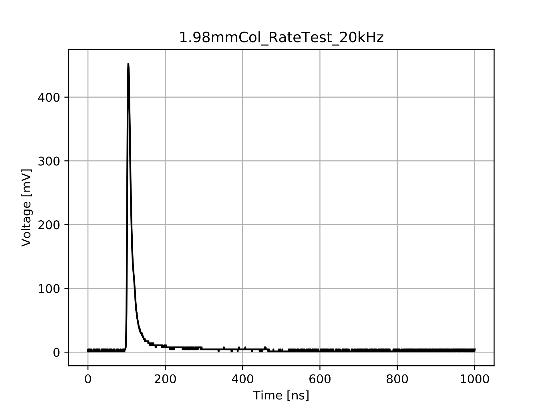
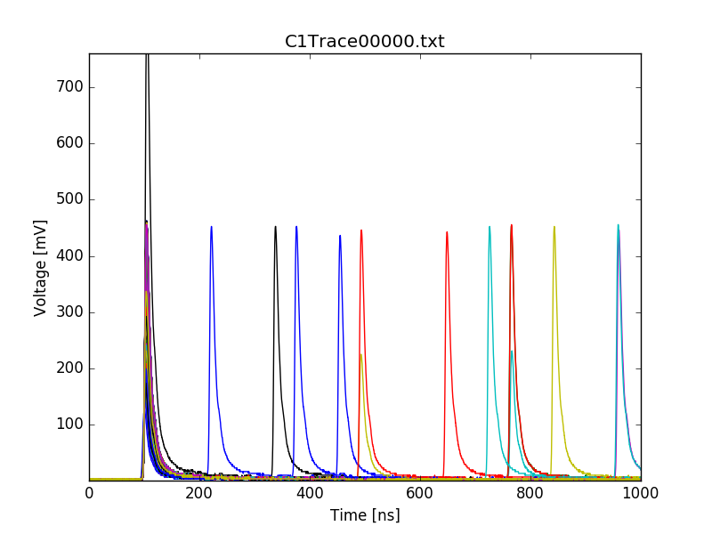
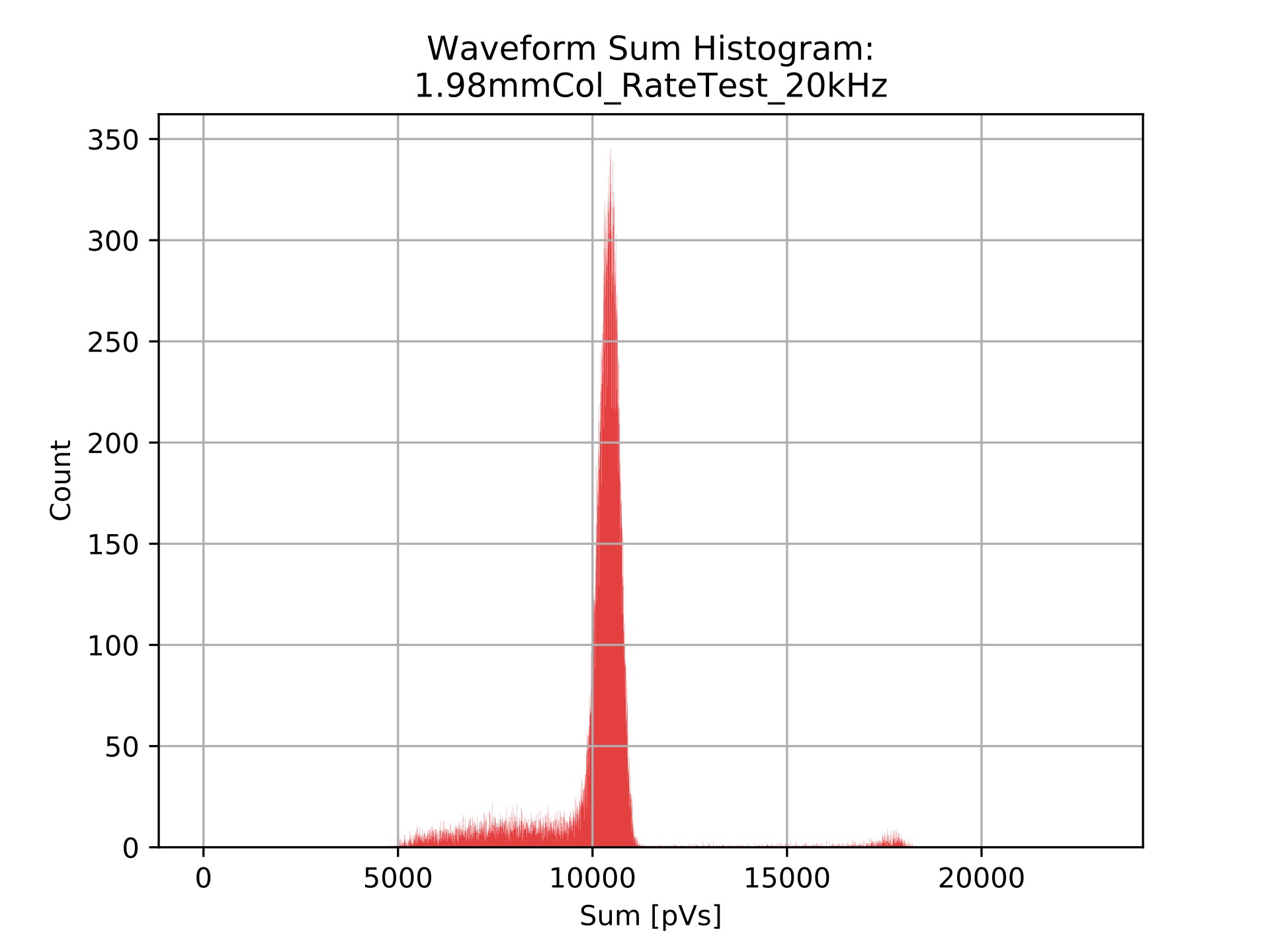
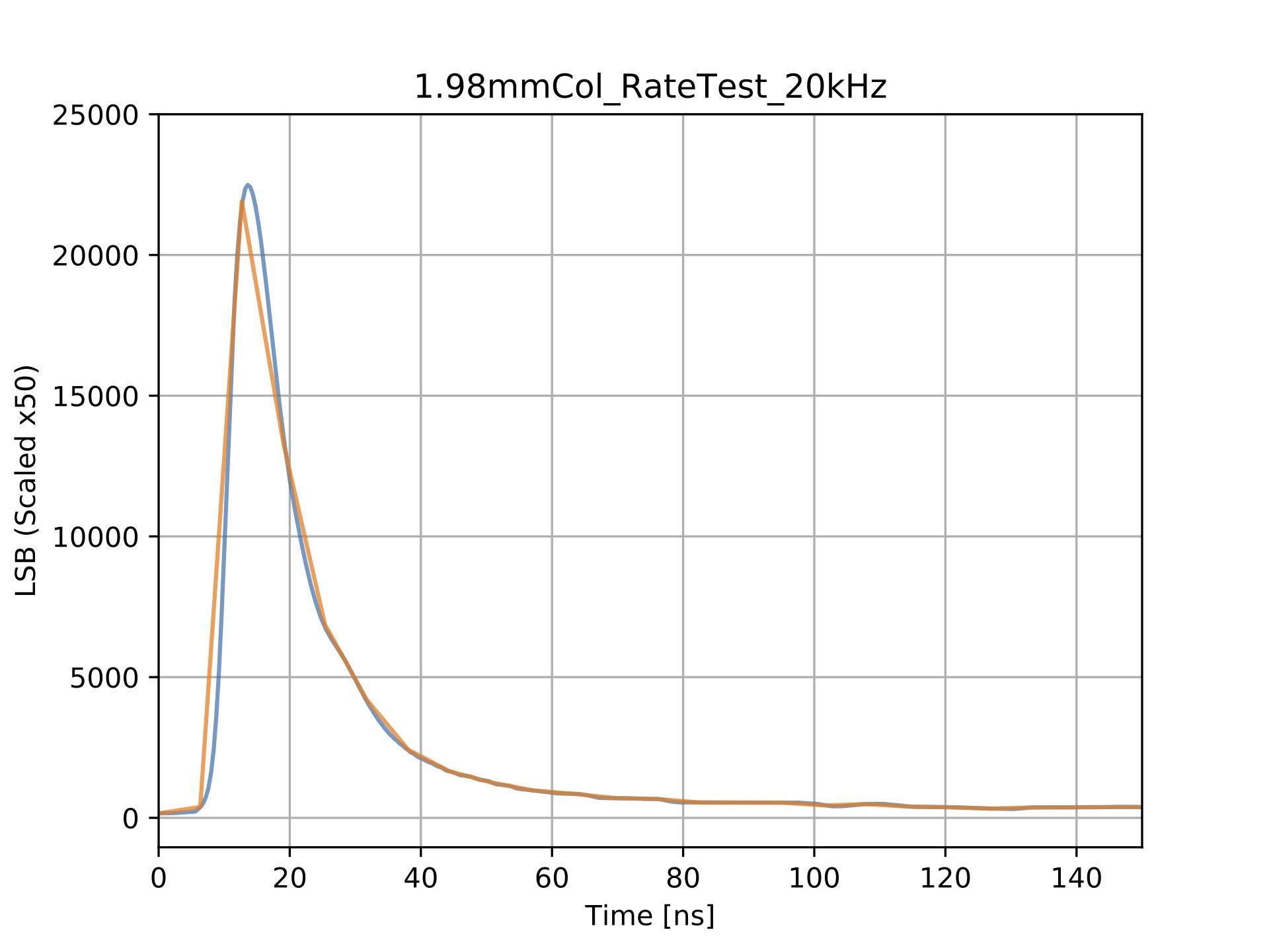
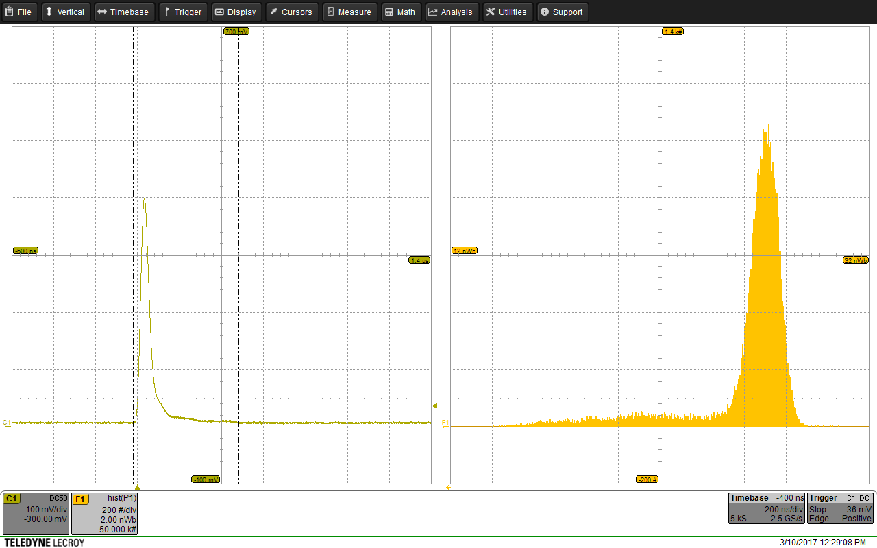
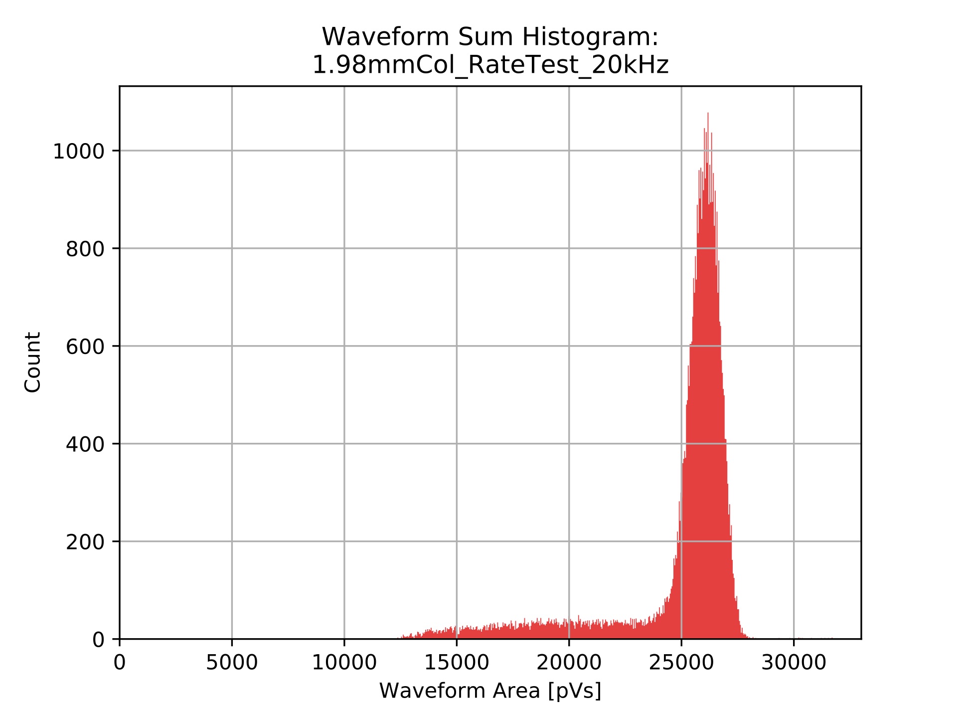
To generate a spectrum for use with the detector emulator, the sample waveforms need to intergrated and put into a histogram. See the figures below shwo an example waveform, a sample of waveforms from a single data file and a generated histogram respectively. If the spectrum is generated as described, from oscilloscope data, the bin width needs to recorded so that the spectrum can be scaled accordingly via the emulator software interface.
Spectrum Modifications
Ideally the method used to create the spectrum should be able to detect bad waveforms, such as those where pile-up has occurred, and discard them so that an "ideal" spectrum is generated. This is so that the these features can be replicated more realistically using the emulator rather than just leaving the artefacts in the spectrum. For example, if the secondary peak from pile-up is in the spectrum, the emulator will take this as part of the “main” spectrum and simply generate pulses with double the area to recreate this secondary peak. To remove some of the bad pulses, a rather primitive method was used to remove that formed part of the spectrum beyond the Gaussian peak and Landau tail. This in effect removed the majority of the additional peaks from pile-up or that were abnormally large.
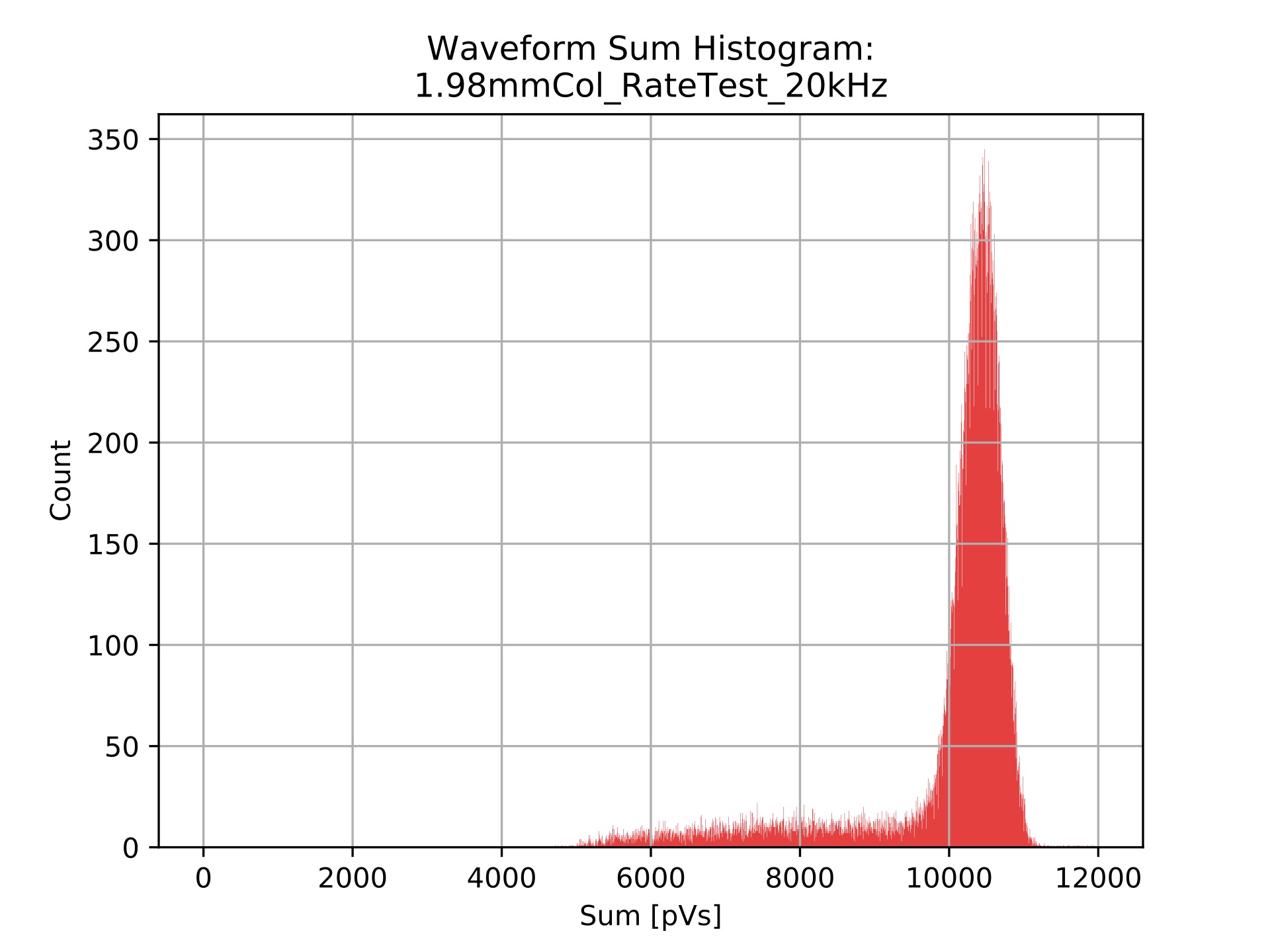
In order for the position of the spectra to be correct, in terms of ADC channel, the file containing the spectral shape needs to start from 0, i.e. if the first populated bin is at 5000 pVs then all prior unpopulated bins from 0 pVs to 5000 pVs need to be included in the spectrum file. Furthermore, it was observed that the x-axis of the spectrum should be scaled using the software interface when importing so that the spectrum is wide enough so that the finer details of the spectrum are reproduced. The simplest two ways to ensure the correct scale along this axis are to either scale by the histogram bin width or to chose a bin width of 1 pVs when producing the spectral histogram. It was found to be best practice not to scale the spectrum along the y-axis (adjusting the peak), as this will exacerbate the features of the spectrum rendering the emulation inaccurate. An example of the adjusted and modified spectrum can be seen in the figure below.
Signal Shape Emulation
The detector emulator allows the user to customise the shape of the output signal pulse. The user can choose to either use the default exponential decay pulse, to define their own custom shape from a list of predefined modifiable inbuilt shapes or shape from an imported .csv file. In addition there is also the ability to generate a multi-shape pulse consisting of two defined signal shapes. In the evaluation of the detector emulator all of the inbuilt signal shapes were tested, these are suitable for simple emulations or in driving additional hardware such as an LED. As one of the aims of the evaluation was to emulate experiential data, an “ideal” waveform was produced from experimental for use with the detector emulator.
Generating an "Ideal" Waveform
Although a signal from a PMT can be roughly characterised using a single or exponential equation, finding the parameters from fitting a function to characterise a typical signal from a specific data set would not straight forward due to the energy/area distribution of the unmodified spectra. Therefore, the chosen method to generate an ideal waveform/signal was to take a selection of “good” waveforms and produce an average signal from them.
In order to do this, what characterised a “good” waveform needed to be defined. Thousands of unique waveforms were recorded per data set, including bad waveforms that would otherwise be rejected, which required the definition to ignore many waveforms. By using the already produced histogram of signal areas, this definition could be relatively simply defined by inspection of the distribution. By inspecting the primary Gaussian shaped peak in the spectrum a short range of waveform areas around the peak could be identified. This, all be it a rather vague and qualitative method, did filter out the majority of bad waveforms, selected only the most common waveforms and selected enough waveforms so that satisfactory average could be produced. This process was all completed via Python script. The averaging function simply generated a single waveform where each point in this waveform was the average of each of the corresponding points in the selected “good” waveforms.
Resolving Resolution Issues
This averaging created a waveform that had the same time resolution as the original data recorded by the oscilloscope which was found to be far finer than what the detector emulator ws able to reproduce. Since the shape file does not have a column representing the time values of each data points, it was necessary to create a new shape file that has the data points from the average waveform mapped onto its coarser time resolution. The resolution/time-step for imported signal shapes is not directly stated in the detector emulator user manual. This was simply calculated by dividing the maximum length a signal shape could be by the maximum number of points that the the signal shape can be defined by and found to be 6.348 ns. A comparison between a ”good” average waveform with the resolution of the oscilloscope and a waveform with the data points mapped to the resolution of the detector emulator can be seen in the figure below.
Changing Units
When importing a custom signal shape into the detector emulator, the signal cannot be defined in terms of volts. Instead it needs to defined in terms of least significant bit (LSB). In the emulator manual the conversion is stated as $\textnormal{LSB} = \frac{4\textnormal{ V}}{2^{16}}$, where the 4 V value refers to the voltage range of out put signals (-2 V to 2 V). However, this conversion was not suitable as the imported spectrum did not have a matching range. Therefore a more general equation was used to find the scale for converting from volts to LSB, $\textnormal{LSB} = \frac{V_{\textnormal{ref}}}{2^{\textnormal{bits}}} = \frac{V_{\textnormal{ref}}}{2^{16}}$, where $V_{\textnormal{ref}}$ is taken as the voltage of most populated bin (this is easiest identified using the detector emulator GUI).
Further Modifications
The imported signal shape was further modified by removing data points (trimming) associated with the dead-time surrounding signal recorded by the oscilloscope (i.e. before trigger and after the pulse). These values which were near to 0 mV (not exactly 0 mV due to dark current) needed to removed so that they were not counted as part of the emulated signal. If left in, this would inhibit the ability to follow the energy spectrum and implement some artificial noise (in particular pile-up). The dark current also had to be subtracted from each of the data points as otherwise, after scaling during emulation, the tail of the signal would form a plateau not tending to 0 mV. The baseline of the average signal was also adjusted so that it was ~0 mV and no longer the opposite polarity of the signal pulse.
Final Scaling
Unfortunately due to how the detector emulator interpolates between data points when gener- ating a signal, there is an averaging effect between points where $\frac{dV}{dt}$ is large and when $\frac{dV}{dt}$ changes polarity quickly. i.e. The emulator struggles to reproduce fine details in an imported shape. This was very significant for the emulation of experimental data as by re-representing the waveform at the lower resolution for the correct length signal to be generated, the short pulse is only defined by a few data points. This then meant that the output signal was significantly smaller than required. Therefore the values in the data file needed to be scaled larger. It is difficult to formally and quantitatively describe by how much an imported signal needs to be scaled by as this depends on how detailed the signal is and its magnitude. The orange trace in Fig.14 shows the final form of a waveform that has had all the necessary steps performed so that it is ready to be emulated.
Time Distribution
The time distribution of signals generated by the detector emulator can be defined by one or four separate methods; at a constant rate, with a Poisson distribution, a custom user defined distribution or custom user defined sequence of events. Since the sample sequence mode on the oscilloscope was used to record record experiential data, the exact rate and time distribution of the experimental data could not be determined. Therefore, for the testing/evaluation of the custom distribution and sequence time distribution modes, arbitrary distributions and sequences were used to verify how these modes worked.
A more in depth evaluation of the constant rate and Poisson time distribution methods was undertaken. These both worked as expected, however it should be noted that the constant rate is defined in terms of kilo counts per second (kcps) where this is equivalent to kHz (i.e. 1 kips ≡ 1 kHz).
Emulator Output
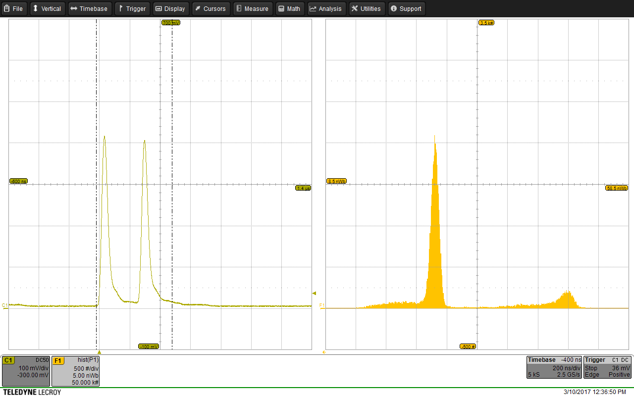
For each iteration of testing the various features of the detector emulator, the signal was output to the Teledyne LeCroy HDO6104 oscilloscope. By using the inbuilt oscilloscope mathematics and graphing functions, it was possible to quickly inspect the output by eye to evaluate if the detector emulator was behaving as expected. The most commonly used inbuilt function/multi-function was to produce an on-the-fly histogram of the signal area. An example of this function in practice can be seen in the figure below, where an acceptable emulation of the experimental data from the 1.98mmCol_RateTest_20kHz run at the Clatterbridge Cancer Centre, 02/08/2016 with all fo the the above described manipulations applied to the spectrum and signal shape.
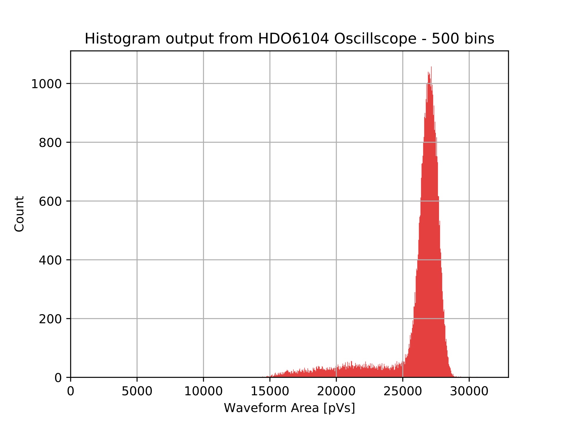
A comparison between the histogram output from the oscilloscope with the corresponding raw binned experimental data (not adjusted for time-step) can be seen in the two figures below, where both histograms have the same bins. Both histograms have the same shape implying the emulation is accurate however it can be seen that the histogram for the experimental data is shifted to the left, this is expected as the integration does not account for the negative baseline voltage and the integration gates are wider. As mentioned earlier, the negative baseline as been taken into account for the emulation, all be it in a relatively crude manner, when generating the average ``good" waveform shape.
Noise and Interference Emulation
Artificial noise and interference can applied to an emulation, this is programmable within the detector emulator software interface. These programmable features are: random number noise, white noise, 1/f noise, baseline drift, random walk, shot noise, interference and pile-up. All types of noise emulation, besides baseline drift and interference, can only be programmed by adjusting one/two variables. Baseline drift can be set by either using the GUI to draw how the baseline changes or by importing a .csv file contain this pattern. Interference is set by importing a .csv file with the interference pattern then choosing the time distribution and magnitude of the interference.
Each of the artificial noise features was individually tested. The feature whose effect can most easily be implemented to replicate experimental data is pile-up. Typically the second (or greater) peak(s) originate from two (or more) pulses falling within the same time window (pile-up). The additional peaks can be re-created by increasing the maximum number of events in pile-up to the number of desired peaks, enabling parallelisation so that multiple pulses can overlap, and reducing the dead-time to 0 ns. An example of this feature being implemented can be seen in figure below.
Unfortunately the user cannot adjust the probability of pile-up occurring, hence making it difficult to change to parameters so that the ratio between the main and additional peaks are correctly replicated as in the spectrum created from the raw data. It should also be noted that if the constant rate time distribution is used, pile-up cannot be emulated.
One could extend the length of the imported signal shape to the length of the oscilloscope recording window minus the trigger offset. This would allow more realistic pile-up to be emulated.
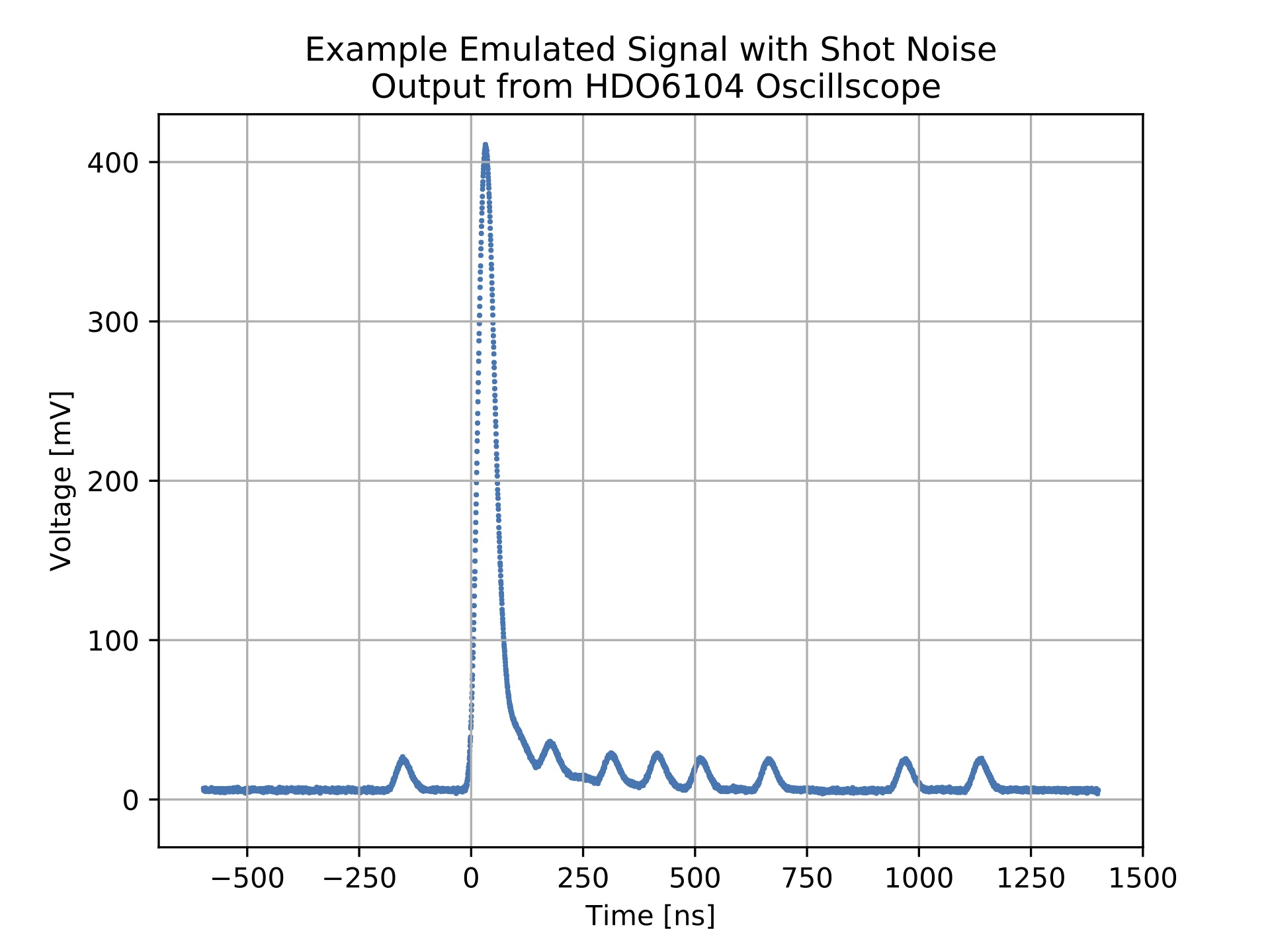
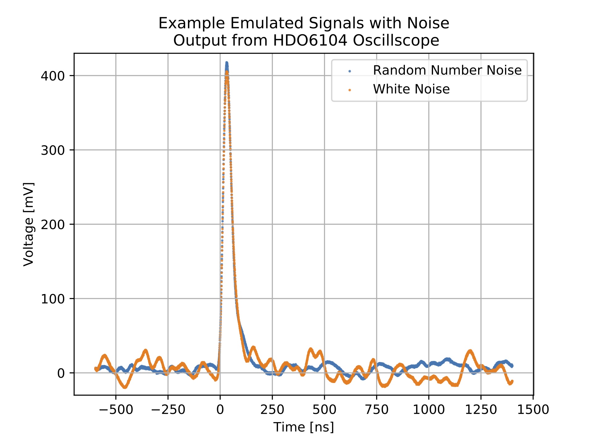
Although a PMT has an associated statistical noise known as shot noise, the shot noise feature in the detector emulator will not produce the same effect and should not be used to emulate this. The artificial shot noise feature of the detector emulator randomly generates Gaussian-like pulses of a user defined magnitude with a user defined probability of occurring. This is not the same thing as PMT shot noise. Instead, the better choice of programmable noise to emulate PMT shot noise would be random number or white noise. These would be more suitable because they are more constant and average (closer) to zero. Whereas emulated shot noise is always the same polarity as the signal. The following two figures show the implementations of shot noise and a random number/white noise compariaon respectively. It may be useful to try and emulate PMT shot/statistical noise because the random fluctuations in the signals is lost in the creation of an average waveform. For this to be effective, the magnitude of the programmed random number or shot noise should be very small relative to the signal amplitude.
Limitations
The main limitation of the DT5800D detector emulator for emulating experimental data of this kind is its ability to generate short and finely detailed pulses. As mentioned before, this is from the relatively coarse resolution of Δt = 6.348 ns between data points for imported signal shapes. This limitation results in a very qualitative trial and error method having to be implemented when scaling the signal shape and a final output signal where the constituent data points can easily be identified.
Another set of limitations, that are more of an inconvenience, are how the some of the features are programmed within the detector emulator software interface. For example not being able to directly specify a probability for pile-up occurring, not being able to change the units in the spectrum display plot from LSB to V but being able to change samples to μs, and that some features sporadically need to selected then deselected and re-selected in order to be implemented.
Evaluation of Potential Uses
Overall the detector emulator is capable of emulating experimental data that is comparable to the original data. Therefore verifying it's suitability for being used to test different methods of data collection and on-the-fly data processing without either having the detector running or using a radiation source. The convenience of being able to do this in a laboratory environment is a particular advantage due to the nature of the application of proton therapy beamlines and their relative scarcity. Every experimental run completed during business hours uses time that could be used ot treat patients which, from a hospital's point of view, is a higher priority.
The accuracy of the emulation is, as mentioned before, limited by the time-step resolution and the qualitative scaling of the signal shape to compensate for the consequences of the resolution. The quality of future emulations could be improved by using a more robust method for identifying and discarding bad waveforms from the ADC (or ADC equivalent) spectrum and a better method for integrating over individual waveforms.
Due to the aforementioned limitations, a better application of the detector emulator may be to use it to drive an LED that injects light into the detector's PMT. Hence, providing another method of stress-testing the detector. This application does not as dependent on the time-step resolution. The detector emulator has been tested and proven to be able to generate the simple pulses that have been previously used to drive an LED in PMT testing. However the stability of the generated signals have not been investigated. Using the detector emulator in role complicates the implementation of programmable noise potential rendering all noise features, bar pile-up, non-applicable.
In the future, if used in conjunction with an improved spectrum, it would be beneficial to investigate how the other programmable noise features could be implemented. This should not be too time intensive as there are not many variables the user can change.
